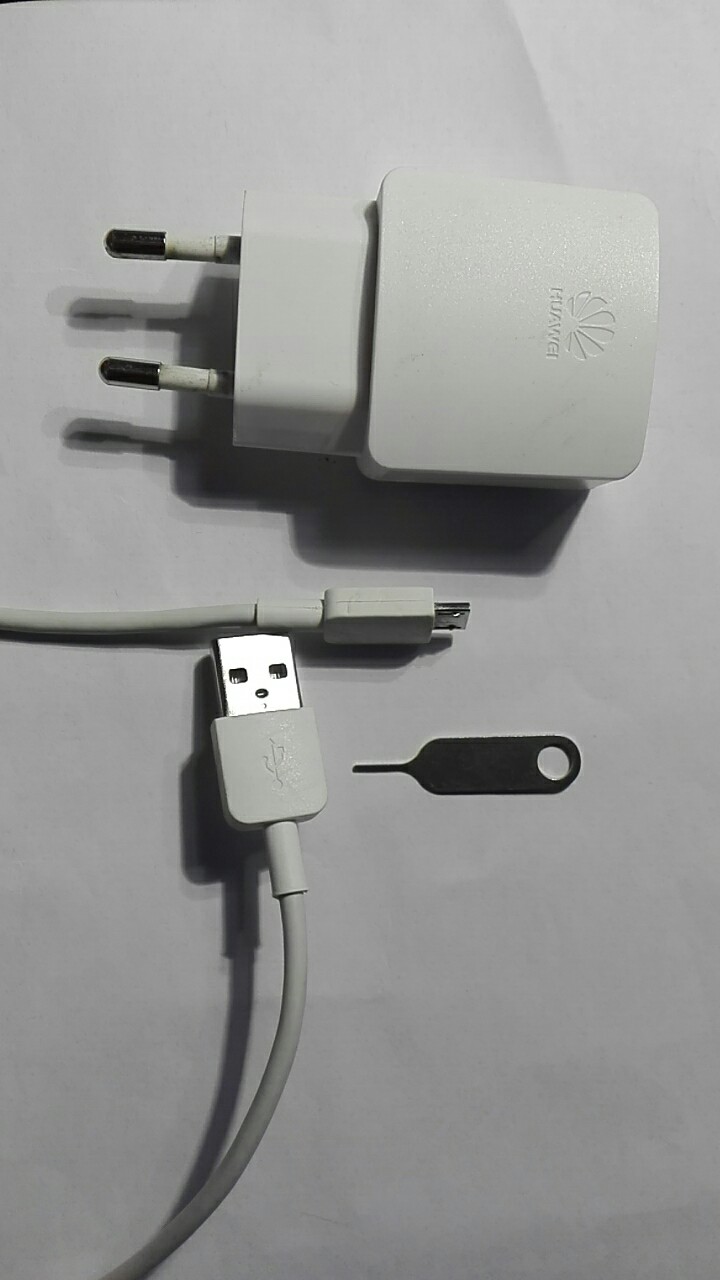
在漫长的等了三天后,290的手机终于从英国伦敦寄到了。
晚上就打开用了。真流畅,还配了壳,预贴了膜!
就是嫌自己的手有些小 😀


My planet
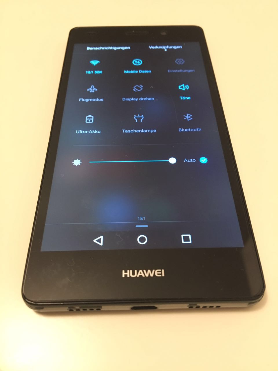
在漫长的等了三天后,290的手机终于从英国伦敦寄到了。
晚上就打开用了。真流畅,还配了壳,预贴了膜!
就是嫌自己的手有些小 😀
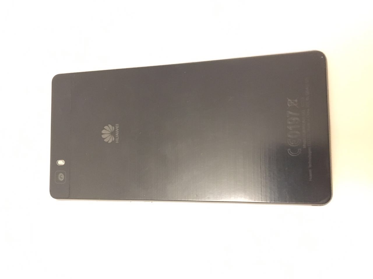
2015年7月13号入手的Huawei P8 Lite被鬼使神差的卖掉了。
剧情真的一曲三折。85放在网上,跟无数买家还价,自己出价82,人没回。后来不想卖了,提价到110,半个小时后系统通知其中一个同意买了,交易成立了。WTF!!!跟客服沟通,未果,告诫他们的系统有严重BUG。
2018.01.10 P8被卖掉了!!!

上周买的Chromecast 2 真好用
旅行之前想象的都很美好,虽然出发时比较痛苦早上4点半的火车。
毅力耐力在开始出发的那一刻开始接受挑战和磨练。


计划周六去儿童图书馆,去自然博物馆。周日上午去中文兴趣班,下午去看赛马。
周六上午出门在图书馆待了一个小时,去博物馆看了半个小时鱼。回家就集体呼呼了。
周日上午去了兴趣班,回家吃了水煮鱼汤面。天气不好,刮风下雨的。又集体呼呼了。
https://support.google.com/adwords/answer/6259715?hl=zh-Hans
最终点击:将促成转化的全部功劳都归于客户最后点击的广告和相应关键字。
首次点击:将促成转化的全部功劳都归于客户首次点击的广告和相应关键字。
线性:将促成转化的功劳平均分配给转化路径上的所有点击。
时间衰减:点击越接近转化发生时间,分配的功劳就越多。点击每相隔七天,所分配的功劳就会相差一半。换言之,转化发生 8 天前的点击所获功劳是转化发生 1 天前的点击所获功劳的一半。
根据位置:向用户首次和最终点击的广告及相应关键字分别分配 40% 的功劳,将其余 20% 的功劳平均分配给转化路径上的其他点击。
以数据为依据:根据转化操作的历史数据来分配促成转化的功劳。(仅供数据充足的帐号使用)
您在中国上海经营一家名为“宝恋”的酒店。一位客户在搜索了“虹口区酒店”、“上海市酒店”、“上海市 3 星级酒店”以及“上海市 3 星级宝恋酒店”这些内容后点击了您的 AdWords 广告,进入了您的网站。她在点击显示“上海市 3 星级宝恋酒店”的广告之后预定了房间。